Comparing maps at different spatial resolutions

Resolution disaggregation, match score, and per-class balanced score, to compare a predicted map to a reference map — in R and in Python.

← Back to tutorials

The problem

Two geomorphological maps obtained at different spatial resolutions cannot be compared cell by cell as they are: the predicted map must first be brought down to the resolution of the reference map, and only then can their agreement be measured — without settling for a single overall score, which would favor majority classes.

The code and functions used here are the ones employed to validate the model presented in “Large-scale mapping” on the Work page. Pick the language you’re interested in below — the method and the results are the same, only the code (and sometimes the figure) differs.

NoteIn short

• The predicted map is disaggregated to recover the resolution of the reference map, cell by cell.
• Match score: proportion of identical cells between the two maps.
• Balanced Match score: average of per-class recalls — each class counts as much as the others, regardless of its frequency.
• In the example below, the balanced score goes from 0.86 to 0.56 depending on how unpredicted cells are counted — that gap alone illustrates why the choice of metric matters.

The method

A study area is delineated then discretized into a grid. The predicted map — produced at a coarser resolution — is disaggregated to recover the resolution of the reference map, and each cell is classified by status: out of area, predicted, or unpredicted.

TipTechnical prerequisites

R packages: ggplot2, dplyr, stringr, sp, sf, ggspatial, ggpubr, ggnewscale, raster. The 4 functions used here (disaggregation, cell status, match score, balanced score) are published separately on Zenodo so they can be reused independently of this notebook.

Functions on Zenodo

library(ggplot2)
library(sp)
library(sf)
library(raster)

# Study area: WGS84 polygon discretized into a grid
crdref <- CRS('+proj=longlat +datum=WGS84')
lon <- c(-116.8, -114.2, -112.9, -111.9, -114.2, -115.4, -117.7)
lat <- c(41.3, 42.9, 42.4, 39.8, 37.9, 38.3, 38.6)
pols <- Polygons(list(Polygon(cbind(lon, lat))), ID = "1")
pols <- SpatialPolygons(list(pols), proj4string = crdref)

ref_sp <- raster(xmn = extent(pols)[1], xmx = extent(pols)[2],
                  ymn = extent(pols)[3], ymx = extent(pols)[4], res = c(.5, .5))
crs(ref_sp) <- crdref

# Reference map (fine resolution, 5 classes) and predicted map (coarse resolution)
r <- raster(xmn = extent(pols)[1], xmx = extent(pols)[2],
            ymn = extent(pols)[3], ymx = extent(pols)[4], res = c(1, 1))
set.seed(12)
values(r) <- sample(1:5, ncell(r), replace = TRUE)
values(ref_sp) <- values(raster::disaggregate(r, fact = 2))
ref_sp_mask <- mask(ref_sp, pols, updateNA = TRUE)

pred_sp <- r
pred_sp[[1]][c(9, 17, 21)] <- c(5, 1, 4)
pred_sp_mask <- mask(pred_sp, pols, updateNA = TRUE)

# Disaggregating the predicted map + cell status (out of area / predicted / unpredicted)
source('disaggregate.R'); source('status-prop.R')
pred_sp_dis <- disagRast(pols, pred_sp_mask, ref_sp, crdref)

ref_spbis <- ref_sp
ref_spbis[is.na(ref_spbis)] <- 999
outstudy <- mask(ref_spbis, pols, updateNA = TRUE)
status <- statusProp(pred_sp_dis, ref_sp, outstudy[[1]], pols, 4326)
PropNL <- status[[4]]  # proportion of unpredicted cells
PropL  <- status[[5]]  # proportion of predicted cells

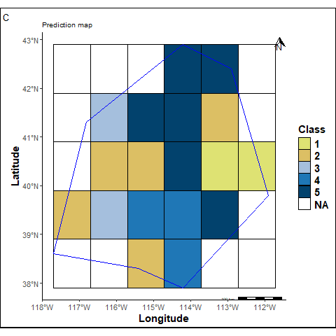
Reference

Predicted

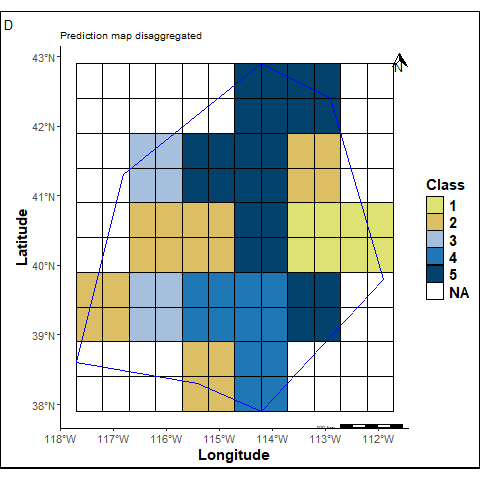
Disaggregated

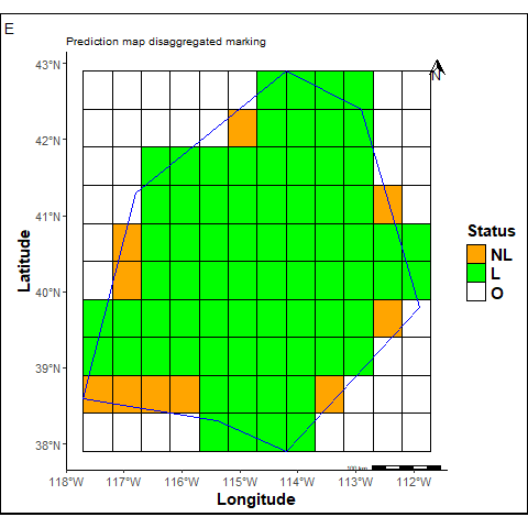
Status

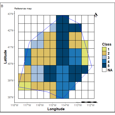
From reference to status map: the predicted map (coarse resolution) is disaggregated to recover the resolution of the reference map, then every cell in the study area is classified as out of area, predicted (green), or unpredicted (orange). In this example, 45 cells are out of area, and of the remaining 82, 72 are predicted (88%) versus 10 unpredicted (12%) — this last proportion is what drives the gap between the raw and corrected scores below.

Disaggregating the predicted map produces edge effects at the periphery of the study area — visible on the status map above.

TipTechnical prerequisites

Only numpy and matplotlib are needed — no geopandas/shapely/rasterio: the point-in-polygon test uses matplotlib.path.Path, and the grids are plain numpy arrays. Full code: compare_maps.py.

import numpy as np
import matplotlib.pyplot as plt
from matplotlib.path import Path
from matplotlib.colors import ListedColormap, BoundaryNorm

# Study area
POLY_LON = [-116.8, -114.2, -112.9, -111.9, -114.2, -115.4, -117.7]
POLY_LAT = [41.3, 42.9, 42.4, 39.8, 37.9, 38.3, 38.6]
POLYGON = np.column_stack([POLY_LON, POLY_LAT])
XMIN, XMAX, YMIN, YMAX = -117.7, -111.9, 37.9, 42.9
NA = np.nan

# Reference map (fine, 10x12) and predicted map (coarse, 5x6)
REFERENCE = np.array([
    [NA, NA, NA, NA, NA, NA,  5,  5, NA, NA, NA, NA],
    [NA, NA, NA, NA, NA,  3,  5,  5,  5,  5, NA, NA],
    [NA, NA, NA,  3,  2,  2,  5,  5,  2,  2, NA, NA],
    [NA, NA,  3,  3,  2,  2,  5,  5,  2,  2,  1, NA],
    [NA,  4,  2,  2,  2,  2,  5,  5,  4,  4,  1, NA],
    [NA,  4,  2,  2,  2,  2,  5,  5,  4,  4,  1, NA],
    [NA,  2,  3,  3,  5,  5,  4,  4,  5,  5,  5, NA],
    [ 2,  2,  3,  3,  5,  5,  4,  4,  5,  5, NA, NA],
    [ 1,  1,  2,  2,  2,  2,  4,  4,  4, NA, NA, NA],
    [NA, NA, NA, NA, NA, NA,  4,  4, NA, NA, NA, NA],
], dtype=float)

PRED_COARSE = np.array([
    [NA, NA, NA,  5,  5, NA],
    [NA,  3,  5,  5,  2, NA],
    [NA,  2,  2,  5,  1,  1],
    [ 2,  3,  4,  4,  5, NA],
    [NA, NA,  2,  4, NA, NA],
], dtype=float)

def cell_polygon_mask(xs, ys, polygon):
    """True for cells whose center lies inside the polygon."""
    xx, yy = np.meshgrid(xs, ys)
    pts = np.column_stack([xx.ravel(), yy.ravel()])
    return Path(polygon).contains_points(pts).reshape(len(ys), len(xs))

def disaggregate(coarse, factor):
    """Disaggregates a coarse grid by repeating each cell factor x factor times."""
    return np.repeat(np.repeat(coarse, factor, axis=0), factor, axis=1)

xs_f = XMIN + 0.5 * (np.arange(12) + 0.5)
ys_f = YMAX - 0.5 * (np.arange(10) + 0.5)
mask_ref = cell_polygon_mask(xs_f, ys_f, POLYGON)

reference = np.where(mask_ref, REFERENCE, np.nan)
predicted = np.where(mask_ref, disaggregate(PRED_COARSE, 2), np.nan)

CLASS_COLORS = ["#dee273", "#dcbf64", "#a5bfdd", "#1f77b6", "#02426d"]

def plot_class(ax, grid, title):
    cmap = ListedColormap(CLASS_COLORS)
    norm = BoundaryNorm(np.arange(0.5, 6.5, 1), cmap.N)
    ax.pcolormesh(np.linspace(XMIN, XMAX, grid.shape[1] + 1),
                  np.linspace(YMAX, YMIN, grid.shape[0] + 1),
                  np.ma.masked_invalid(grid), cmap=cmap, norm=norm,
                  edgecolors="black", linewidth=0.3)
    ax.plot(np.append(POLY_LON, POLY_LON[0]), np.append(POLY_LAT, POLY_LAT[0]), color="blue", linewidth=1)
    ax.set_title(title, fontsize=10)
    ax.set_xticks([]); ax.set_yticks([])

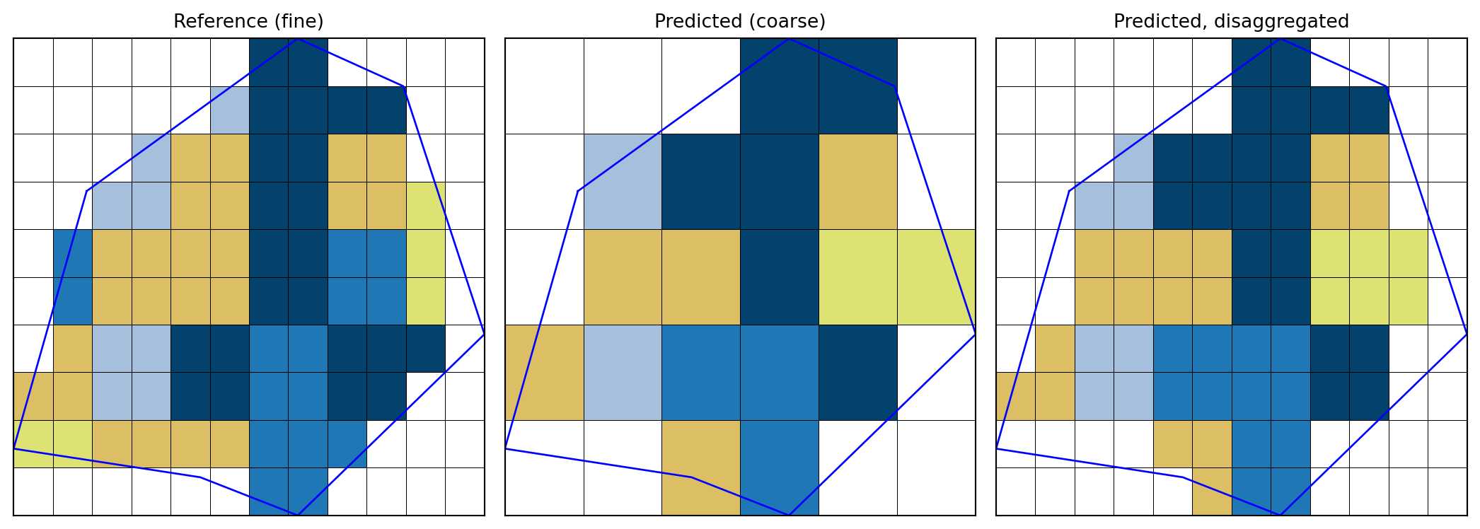
fig, axes = plt.subplots(1, 3, figsize=(11, 4))
plot_class(axes[0], reference, "Reference (fine)")
plot_class(axes[1], PRED_COARSE, "Predicted (coarse)")
plot_class(axes[2], predicted, "Predicted, disaggregated")
fig.tight_layout()
plt.show()

Figure 1: From reference to disaggregated predicted map

The results

Two families of scores measure agreement between the two maps: a simple match score (proportion of identical cells), and a per-class balanced score that neutralizes the effect of dominant classes (per Grandini et al. 2020). Each comes in an uncorrected version (which ignores unpredicted cells) and one or two corrected versions (which count them as errors, more or less severely).

Score	Value	What it measures
Match — uncorrected	0.82	Identical cells, unpredicted cells ignored
Match — corrected	0.71	Same, unpredicted cells counted as errors
Balanced Match — raw (NCBM)	0.86	Average of per-class recalls, unpredicted cells ignored
Balanced Match — corrected, prop. 1	0.76	NCBM penalized by the proportion of unpredicted cells
Balanced Match — corrected, prop. 2	0.56	Unpredicted cells reintegrated, recall set to 0

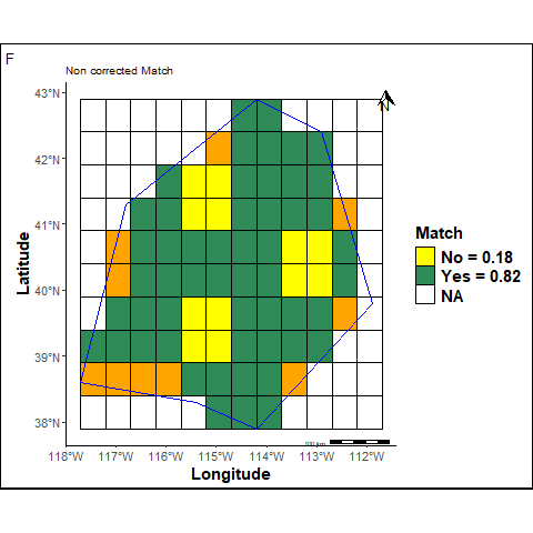
Uncorrected match

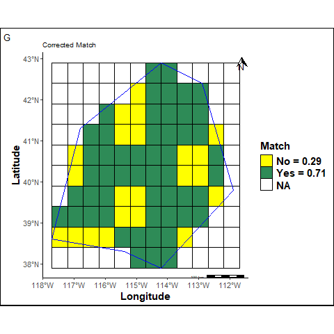
Corrected match

def match_score(pred, ref, mask, correct=False):
    valid_ref = mask & ~np.isnan(ref)
    if correct:
        return float((valid_ref & (pred == ref)).sum() / valid_ref.sum())
    valid = valid_ref & ~np.isnan(pred)
    return float(np.mean(pred[valid] == ref[valid]))

def balanced_match(pred, ref, mask, classes):
    valid_ref = mask & ~np.isnan(ref)
    valid_pred = valid_ref & ~np.isnan(pred)
    recalls_ncbm, recalls_cbm2 = [], []
    for k in classes:
        idx_pred = valid_pred & (ref == k)
        if idx_pred.sum() > 0:
            recalls_ncbm.append(float((idx_pred & (pred == k)).sum() / idx_pred.sum()))
        idx_ref = valid_ref & (ref == k)
        if idx_ref.sum() > 0:
            recalls_cbm2.append(float((idx_ref & (pred == k)).sum() / idx_ref.sum()))
    n_L = (mask & ~np.isnan(pred)).sum()
    n_NL = (mask & np.isnan(pred) & ~np.isnan(ref)).sum()
    ncbm = float(np.mean(recalls_ncbm))
    cbm1 = ncbm * (n_L / (n_L + n_NL))
    cbm2 = float(sum(recalls_cbm2) / (len(recalls_cbm2) + 1))
    return ncbm, cbm1, cbm2

match_nc = match_score(predicted, reference, mask_ref, correct=False)
match_c = match_score(predicted, reference, mask_ref, correct=True)
ncbm, cbm1, cbm2 = balanced_match(predicted, reference, mask_ref, [1, 2, 3, 4, 5])

print(f"Uncorrected match : {match_nc:.2f}")
print(f"Corrected match    : {match_c:.2f}")
print(f"NCBM (raw)         : {ncbm:.2f}")
print(f"CBM1 (corrected, prop. 1) : {cbm1:.2f}")
print(f"CBM2 (corrected, prop. 2) : {cbm2:.2f}")

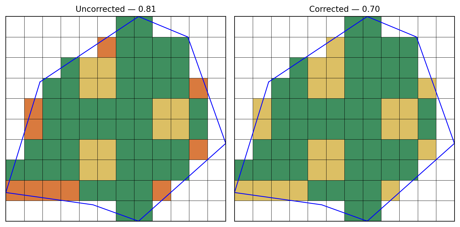
Uncorrected match : 0.81
Corrected match    : 0.70
NCBM (raw)         : 0.86
CBM1 (corrected, prop. 1) : 0.74
CBM2 (corrected, prop. 2) : 0.56

Score	Value	What it measures
Match — uncorrected	0.81	Identical cells, unpredicted cells ignored
Match — corrected	0.70	Same, unpredicted cells counted as errors
Balanced Match — raw (NCBM)	0.86	Average of per-class recalls, unpredicted cells ignored
Balanced Match — corrected, prop. 1	0.74	NCBM penalized by the proportion of unpredicted cells
Balanced Match — corrected, prop. 2	0.56	Unpredicted cells reintegrated, recall set to 0

valid_ref = mask_ref & ~np.isnan(reference)
predicted_here = ~np.isnan(predicted)

cat_nc = np.full(reference.shape, np.nan)
cat_nc[valid_ref & predicted_here & (predicted == reference)] = 1
cat_nc[valid_ref & predicted_here & (predicted != reference)] = 0
cat_nc[valid_ref & ~predicted_here] = 2

cat_c = np.where(valid_ref, 0.0, np.nan)
cat_c[valid_ref & predicted_here & (predicted == reference)] = 1

def plot_match(ax, grid, colors, bounds, title):
    cmap = ListedColormap(colors)
    norm = BoundaryNorm(bounds, cmap.N)
    ax.pcolormesh(np.linspace(XMIN, XMAX, grid.shape[1] + 1),
                  np.linspace(YMAX, YMIN, grid.shape[0] + 1),
                  np.ma.masked_invalid(grid), cmap=cmap, norm=norm,
                  edgecolors="black", linewidth=0.3)
    ax.plot(np.append(POLY_LON, POLY_LON[0]), np.append(POLY_LAT, POLY_LAT[0]), color="blue", linewidth=1)
    ax.set_title(title, fontsize=10)
    ax.set_xticks([]); ax.set_yticks([])

fig, axes = plt.subplots(1, 2, figsize=(8, 4))
plot_match(axes[0], cat_nc, ["#dcbf64", "#3f8f5f", "#d97a3e"], [-0.5, 0.5, 1.5, 2.5],
           f"Uncorrected — {match_nc:.2f}")
plot_match(axes[1], cat_c, ["#dcbf64", "#3f8f5f"], [-0.5, 0.5, 1.5],
           f"Corrected — {match_c:.2f}")
fig.tight_layout()
plt.show()

Figure 2: Uncorrected (left) and corrected (right) match

These five numbers measure the same predicted map, but answer different questions: how accurate am I where I predicted? (uncorrected versions) versus how accurate am I given everything I didn’t predict? (corrected versions). The right score depends on the intended use, not on a universal convention.

TipMathematical detail

\[ Match\ (Yes) = \frac{N_{+}}{N_{+} + N_{-}} \qquad\qquad Recall_{k} = \frac{TP_{k}}{TP_{k} + FN_{k}} \]

\[ NCBM = \frac{1}{K}\sum_{k=1}^{K} Recall_{k} \qquad CBM_{1} = NCBM \times (1 - \%NL) \qquad CBM_{2} = \frac{1}{K}\sum_{k \neq 99}^{K} Recall_{k} \]

where \(N_{+}\)/\(N_{-}\) are cells with identical/different classes between the two maps, and \(K\) is the number of classes (5 for NCBM and CBM₁, 6 for CBM₂ which reintegrates the unpredicted-cell class, with recall conventionally set to 0).

Try it yourself

The actual computation above relies on structures too heavy to run directly in a browser (sf/raster in R, a fine grid in Python). Here is a simplified version on a small 4×4, 3-class example: edit the values of pred below and click Run to see the scores change — executed directly in your browser, no server involved.

Warning

Simplified version for teaching purposes, on a small toy example — the real computation on full maps is the one from the previous section.

NoteWhat this code does

ref and pred are two small 4×4, 3-class grids (reference and prediction). match_score computes the proportion of identical cells between the two; balanced_match averages the recalls class by class, so the most frequent class can’t dominate the score — these are the same two functions as above, reduced to their essentials. Change a few values of pred and rerun to see the two scores move differently.

NoteWhat this code does

ref and pred are two small 4×4, 3-class grids (reference and prediction). match_score computes the proportion of identical cells between the two; balanced_match averages the recalls class by class, so the most frequent class can’t dominate the score — these are the same two functions as above, reduced to their essentials. Change a few values of pred and rerun to see the two scores move differently.

Go further

R code on GitHub Python code on GitHub Functions on Zenodo View the “Large-scale mapping” project Back to tutorials

This method was used to validate the automatic geomorphological mapping model described in Faye et al. (2024).

Faye, Paul Aimé Latsouck, Elodie Brunel, Thomas Claverie, Solym Mawaki Manou-Abi, and Sophie Dabo-Niang. 2024. “Automatic Geomorphological Mapping Using Ground Truth Data with Coverage Sampling and Random Forest Algorithms.” Earth Science Informatics 17 (4): 3715–32.

Grandini, Margherita, Enrico Bagli, and Giorgio Visani. 2020. “Metrics for Multi-Class Classification: An Overview.” arXiv Preprint arXiv:2008.05756.