Choosing where to sample in the field is not a trivial matter: simple random sampling can over-represent some zones and leave others completely absent, especially when the study area is irregular. What’s needed is a sampling design that guarantees homogeneous spatial coverage — or, better still, that concentrates effort where the terrain is most complex, and therefore hardest to predict.
The code and functions used here are the ones employed to build the training data for the model described in “Large-scale mapping” on the Work page, applied to a real reef area (the Geyser bank, off Mayotte). The method and results are the same in R and Python — pick your language down at the code, a bit further below.
NoteIn short
SCS-KMeans: k-means on the coordinates of a regular grid — uniform coverage, sampled points are the cluster centers.
SCS-CLARA: same goal, but each sampled point is an actual cell of the terrain (its medoid), not a computed center — this is the CLARA/PAM algorithm in R.
CDS-CLARA(complexity-dependent): clustering is done on terrain depth and roughness rather than on coordinates — sampling concentrates where the relief is most complex.
The method
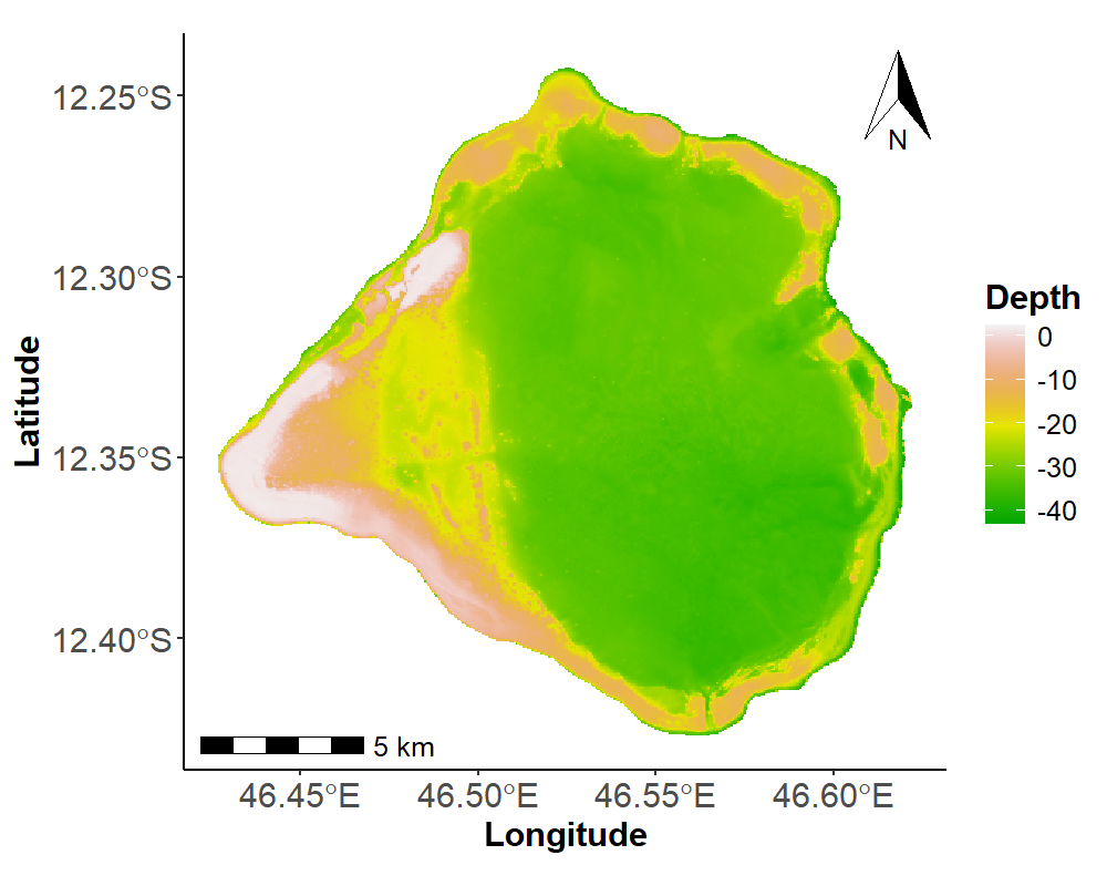
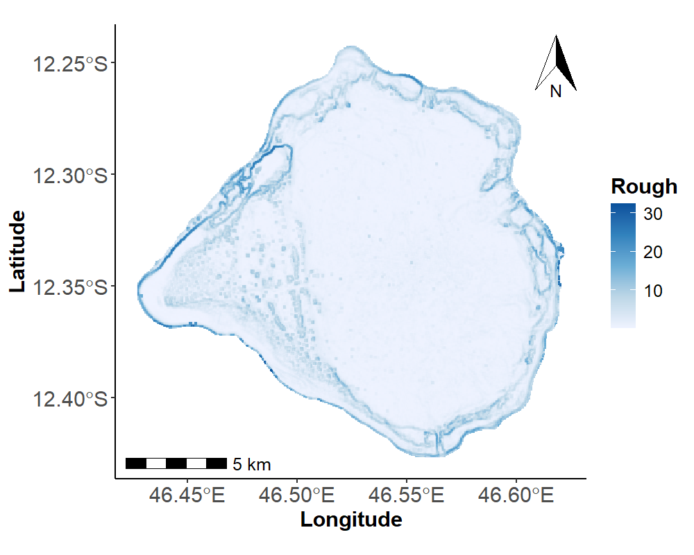
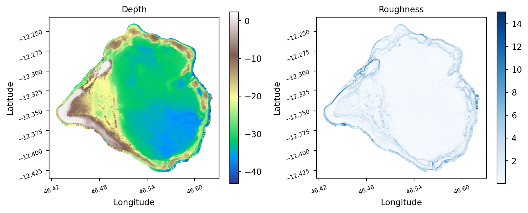
The terrain is described by a real raster at 50 m resolution (depth and roughness, among other variables), on which the three methods are applied.
See the code and results in
TipTechnical prerequisites
R packages: raster, terra, sf, sp, ggplot2, ggspatial, ggnewscale. The functions scsKM, scsCLARA, cdCLARA, and plotPoints are published separately on Zenodo.
library(raster)library(sf)library(ggplot2)library(ggspatial)library(ggnewscale)source("scs-kmeans.R") # scsKM() : k-means on coordinatessource("scs-clara.R") # scsCLARA(): medoids (CLARA) on coordinatessource("cd-clara.R") # cdCLARA() : medoids (CLARA) on depth + roughnesssource("sample-points-plot.R")# Real terrain raster (50 m resolution): depth, roughness, ...Terrain_Attr_50 <- terra::rast("50m_rast_Attr2.tif")Terrain_Attr_50_df <-as.data.frame(Terrain_Attr_50, xy =TRUE)names(Terrain_Attr_50_df) <-append(c("Longitude", "Latitude"), all_predicteurs)Depth_plot <-ggplot(shp2) +geom_sf(fill =NA, color =NA) +geom_tile(data = Terrain_Attr_50_df, aes(Longitude, Latitude, fill = Prof_Moyenne)) +scale_fill_gradientn(colours =terrain.colors(100), na.value ="white", name ="Depth")Roughness_plot <-ggplot(shp2) +geom_sf(fill =NA, color =NA) +geom_tile(data = Terrain_Attr_50_df, aes(Longitude, Latitude, fill = rough)) +scale_fill_gradientn("Rough", colours = RColorBrewer::brewer.pal(5, "Blues"), na.value ="gray")
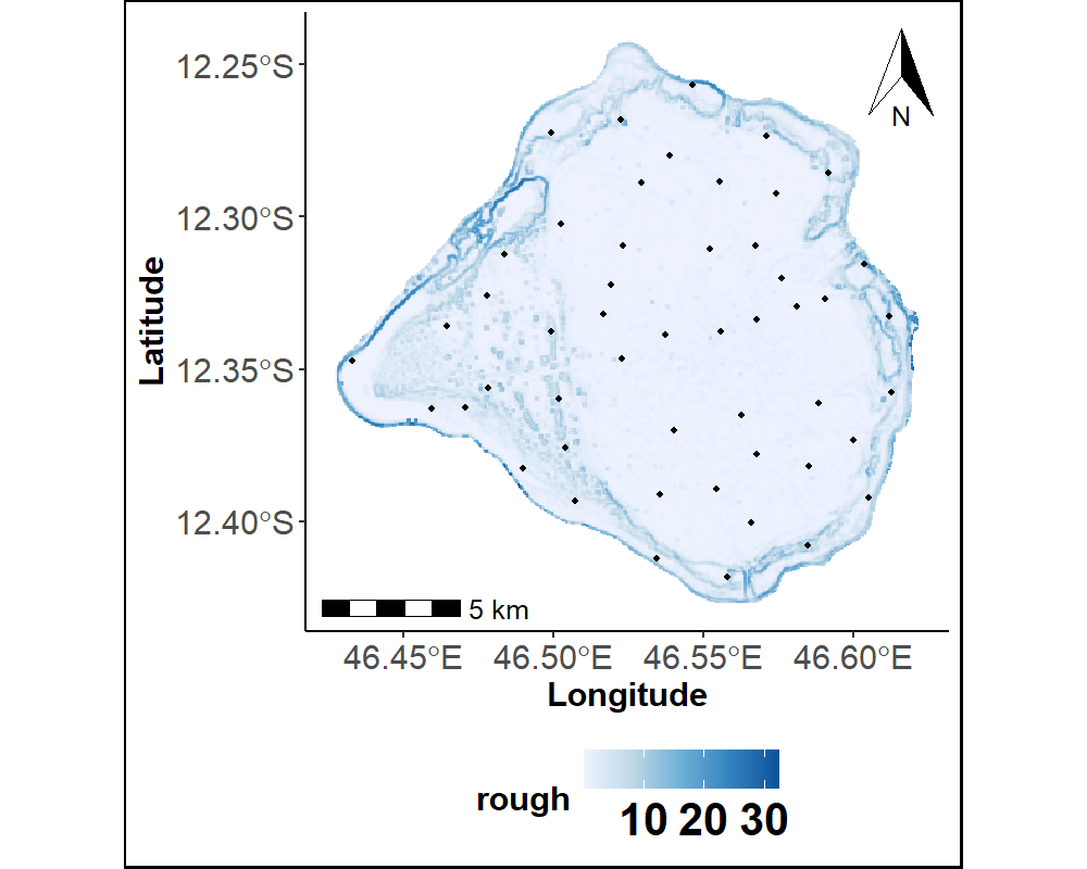
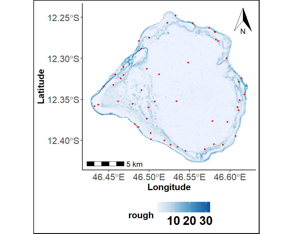
Depth
Roughness
These two variables — depth and roughness — describe the complexity of the relief: they are what CDS-CLARA sampling is based on, while SCS-KMeans and SCS-CLARA ignore the relief and only consider geographic position.
TipTechnical prerequisites
Only numpy, matplotlib, and scikit-learn are needed. The source raster is an LZW-compressed multi-band GeoTIFF, unreadable by the usual geospatial libraries unavailable here (rasterio, GDAL) — a small pure-Python TIFF/LZW reader handles it instead. Full code: terrain_reader.py, sampling.py.
Show code
import syssys.path.insert(0, ".")import numpy as npimport matplotlib.pyplot as pltfrom terrain_reader import read_tiff_bands, read_geotransform, utm_to_latlon# Real terrain raster (50 m resolution, 9 bands): band 0 = depth, band 1 = roughnessbands = read_tiff_bands("50m_rast_Attr2.tif")depth, rough = bands[0], bands[1]H, W = depth.shape# Real georeferencing (UTM 38S), read from the GeoTIFF's own tags: row 0 is northscale_x, scale_y, tie_x, tie_y = read_geotransform("50m_rast_Attr2.tif")rows, cols = np.mgrid[0:H, 0:W]EASTING, NORTHING = tie_x + cols * scale_x, tie_y - rows * scale_yLAT, LON = utm_to_latlon(EASTING, NORTHING)valid =~np.isnan(depth) &~np.isnan(rough)coords = np.column_stack([EASTING[valid], NORTHING[valid]]) # UTM meters, for clusteringlonlat = np.column_stack([LON[valid], LAT[valid]]) # degrees, for displaycomplexity = np.column_stack([depth[valid], rough[valid]])
Figure 1: Depth and roughness of the real terrain (Geyser bank)
The results
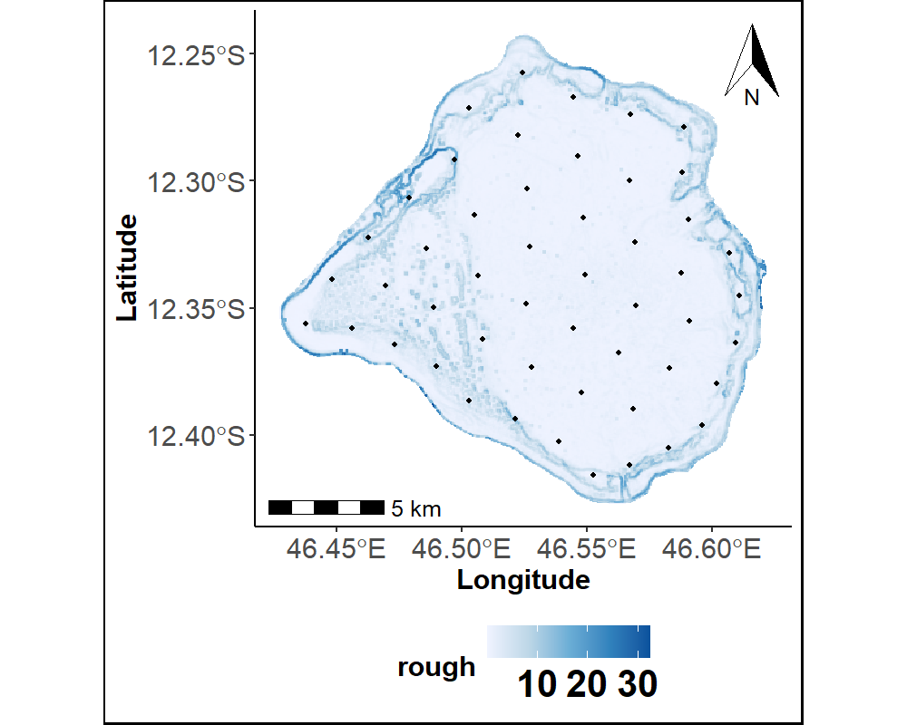
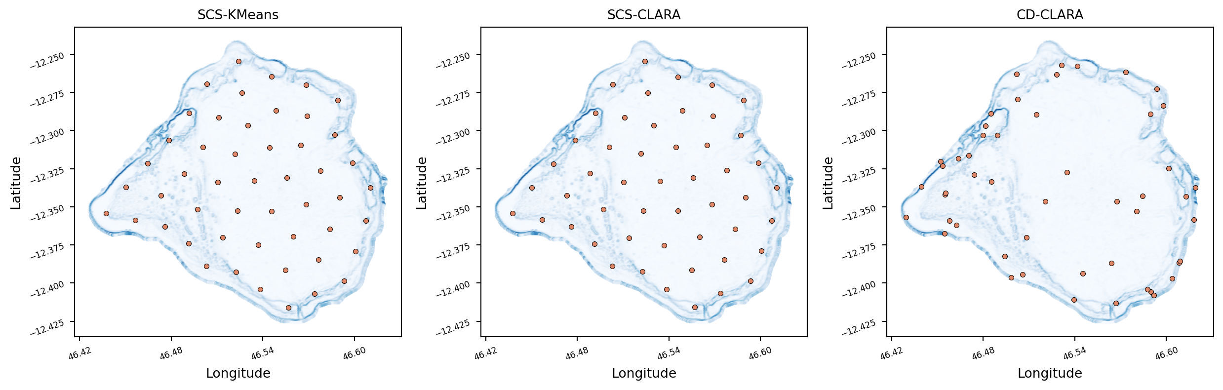
The three methods are applied to the same area, with the same number of sampled points (K = 50), but different criteria: covering the space uniformly, or concentrating on complex relief.
pvtscskm <-scsKM(shp = Geyser_bathy, var =c("Longitude", "Latitude"),iter =12, sampsize =50, nT =10)pvtscscl <-scsCLARA(data = Terrain_Attr_50_df, var =c("Longitude", "Latitude"),iter =1, sampsize =50, disT ="euclidean")pvtcdcl <-cdCLARA(data = Terrain_Attr_50_df, var1 =c("Longitude", "Latitude"),var2 =c("Prof_Moyenne", "rough"), iter =12, sampsize =50, disT ="manhattan")
SCS-KMeans
SCS-CLARA
CDS-CLARA
The first two methods produce a grid of points regularly spaced across the whole area. The third departs from that clearly: points cluster along the edges, where roughness is highest.
Figure 2: Points sampled by the three methods, over a roughness background
The first two methods produce a grid of points regularly spaced across the whole area. The third departs from that clearly: points cluster along the edges, where roughness is highest.
where \(x_i\) are the terrain cells and \(c_k\) the \(K\) sampled points: k-means chooses the \(c_k\) that minimize the average squared distance to the nearest sampled point — hence the regular coverage. SCS-CLARA and CDS-CLARA use this same criterion, but additionally require each \(c_k\) to be an actual cell of the terrain (a medoid), not a recomputed center.
Try it yourself
The actual computation above covers over 100,000 cells — too many for a browser. Here is the same idea on a small cloud of 16 points in 2D, grouped into 3 visually distinct clusters: change k and click Run to see which points get chosen as samples.
Warning
Simplified version for teaching purposes, on a toy example — the real computation on the full data is the one from the previous section.
NoteWhat this code does
16 2D points are grouped into k clusters: the algorithm alternates between assigning each point to its nearest center and recomputing the centers, until convergence — then, for each cluster, keeps the actual observed point closest to its center (the medoid), rather than the center itself, which is generally not a point in the dataset. Change k and rerun to see the clustering adapt.
NoteWhat this code does
16 2D points are grouped into k clusters: the algorithm alternates between assigning each point to its nearest center and recomputing the centers, until convergence — then, for each cluster, keeps the actual observed point closest to its center (the medoid), rather than the center itself, which is generally not a point in the dataset. Change k and rerun to see the clustering adapt.
These sampling methods were used to build the training data for the automatic geomorphological mapping model described in Faye et al. (2024).
Bibliography
Faye, Paul Aimé Latsouck, Elodie Brunel, Thomas Claverie, Solym Mawaki Manou-Abi, and Sophie Dabo-Niang. 2024. “Automatic Geomorphological Mapping Using Ground Truth Data with Coverage Sampling and Random Forest Algorithms.”Earth Science Informatics, 1–18.